How to Protect Formulas in Cells
To protect a formula, simply right-click on one or more cells containing the formulas you want to hide and select “Protect selected cell(s) with XLS Padlock” from the context menu.
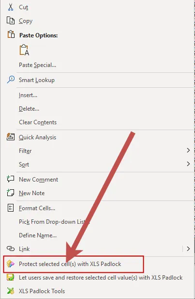
XLS Padlock will then confirm that the cells are marked for protection.
Overview of Protected Cells
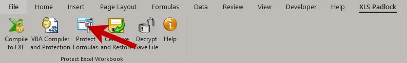
Section titled “Overview of Protected Cells”To see an overview of all protected cells, click “Protect Formulas” in the XLS Padlock tab or menu:
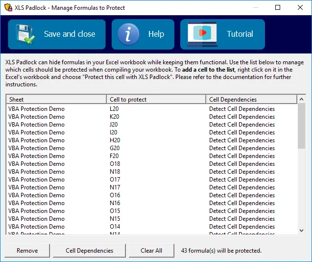
This opens a list of all cells configured for protection. In this window, you can adjust protection behavior, remove protection from specific cells, or clear the entire list.
When you compile your workbook, XLS Padlock replaces all listed formulas with generic function calls like PLEvalForm(N) and PLEvalFormD(N, ….). Your cells remain functional, but end-users cannot discover the underlying formulas. The original formulas no longer exist in the compiled workbook; they are managed by the EXE itself.
Cell Dependencies
Section titled “Cell Dependencies”The Cell Dependencies button lets you control how protection is applied. Two choices are available: “Detect Cell Dependencies” and “No”.
By default, XLS Padlock will detect all cell references and range names in your formulas (cell dependencies) and generate an anonymous function that contains these references. This allows Excel to recalculate protected cells properly. For instance, if the formula to protect is =A3^2, XLS Padlock will generate a function like: PLEvalFormD(1, COUNT(A3)).
If XLS Padlock fails to protect a cell, you can choose “No” for its “Cell Dependencies” setting. In this case, a simple generic PLEvalForm(N) function will be used.
👉 See also